Machine Learning: End-to-end Classification
In machine learning, classification is the task of predicting the class of an object out of a finite number of classes, given some input labeled dataset. In this tutorial, you’ll learn how to pre-process your training data, evaluate your classifier, and optimize it. By Mikael Konutgan.
Training and Cross Validation
Now that the data is ready, you can create a classifier and train it. Add the following code to a new cell:
X = credit_[["Age", "Education", "Student", "Married"]]
y = credit_["Creditworthy"]

X_train, X_test, y_train, y_test = train_test_split(X, y, test_size=0.5, random_state=RANDOM_STATE)
You're selecting four of the features on which to train the model, and you are storing them in X. The Creditworthy column is your target, named y.
In the final line, you're splitting the dataset into two random halves, a training set to train the classifier on, and a testing set to validate the classifier to see how well you did. You can learn more about this process in the Beginning Machine Learning tutorial.
Next, add the following code to a new cell:
estimator = LogisticRegression(random_state=RANDOM_STATE)  # 1
estimator.fit(X_train, y_train)  # 2

y_true = y_test  # 3
y_pred = estimator.predict(X_test)  # 4
y_score = estimator.predict_proba(X_test)[:, 0]  # 5
There's a lot going on here:
- You use logistic regression as the classifier. The details behind it are out of scope for this tutorial. You can learn more about this in this wonderful picture guide.
- You train — or "fit" — the classifier on the training part of the dataset.
-
y_truewill hold the true value of theycolumn that is the creditworthiness value. In this case, it's just the test values themselves. -
y_predholds the predicted new values of the creditworthiness. You'll use this value along with the true values to evaluate the performance of your classifier shortly. Note that this evaluation is done with the test set, because the classifier hasn't 'seen' these yet, and the goal is to predict unknown values. Otherwise, you could've just memorized the training values and predicted everything correctly every time. - Logistic regression is a classification algorithm that actually predicts a probability. The output of the model is something like: "The probability that the person with the given values is creditworthy is 75%." You can use these probability scores to evaluate more advanced metrics of the classifier.
You've successfully trained the classifier and used it to predict a probability! Next, you'll find out how well you did.
Accuracy
One of the simplest metrics to check how well you did is the accuracy of your model. What percentage of the values can the classifier predict correctly?
Add this line to a new cell:
accuracy_score(y_true=y_true, y_pred=y_pred)
accuracy_score takes your y column true and predicted values and returns the accuracy. Run the cell and check the results:
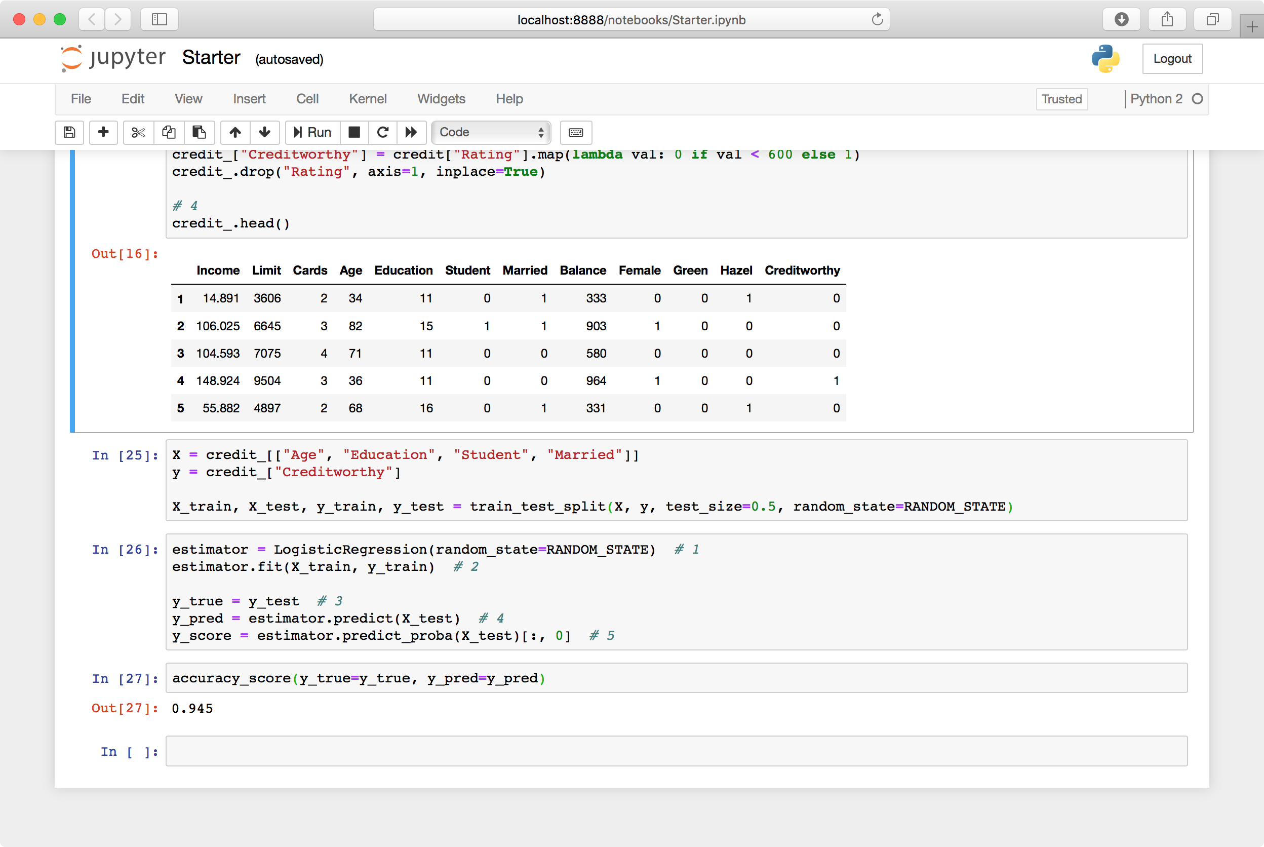
Almost 95%! Did you really do that well with just the age, education, student and marriage status of a person?
It turns out that out of the 200 rows in the testing dataset, only 11 of the rows are creditworthy. This means that a classifier that always predicts that the row is not creditworthy also has an accuracy of about 95%!
So the 95% your classifier predicted isn't that good — or any good actually. The accuracy, though often useful when the different classes are balanced, can be very misleading out of context. A better metric, or family of metrics, and one you should always look at, is the confusion matrix.
Understanding Confusion Matrix, Precision and Recall
A confusion matrix plots true values against predicted values. Precision and recall are two extremely useful metrics derived from a confusion matrix. In the context of your dataset, the metrics answer the following questions:
- Precision: Out of all of the people who were creditworthy, what percentage of them were correctly predicted to be creditworthy?
- Recall: Out of all of the people who were predicted to be creditworthy, what percentage of them were actually creditworthy?
This will become a bit clearer when you see the data, so it's time to add some code. Create new cells for each of the following code blocks and run them all (don't worry about the warning):
confusion_matrix(y_true=y_true, y_pred=y_pred)
precision_score(y_true=y_true, y_pred=y_pred)
recall_score(y_true=y_true, y_pred=y_pred)
plot_confusion_matrix(cm=confusion_matrix(y_true=y_true, y_pred=y_pred),
                      class_names=["not creditworthy", "creditworthy"])

In the first cell, confusion_matrix plots the true values against the predicted values. Each quadrant in the output multi-dimensional array represents a combination of a true value and a predicted value. For example, the top-right is the number of rows that were not creditworthy and were also correctly predicted by your classifier to be not creditworthy.
The last cell includes a visualization of this, wherein each quadrant was also divided by the total number of rows. You can see that your current classifier is actually doing what you feared it was doing: It's just predicting all the rows to be not creditworthy.
In the middle, you'll see calculations for precision_score and recall_score. Both of these metrics range from 0 (0%) to 1 (100%). The closer you are to 1, the better. There's always a tradeoff between these two metrics.
For example, if you weren't as strict with your credit check, and you let some questionable people through, you would increase your precision, but your recall would suffer. On the other hand, if you were extremely strict, your recall might be impeccable, but you would fail to hand out credit to many creditworthy individuals, and your precision would suffer. The exact balance you need will depend on your use case.
Both your precision and your recall are 0, indicating that the classifier is currently quite terrible. Go back to the cell wherein you set X and y, and change X to the following:
X = credit_[["Income", "Education", "Student", "Married"]]
You're now using the Income value as part of the training. Go to Kernel ▸ Restart & Run All to re-run all of your cells.

The precision has increased to 0.64, and the recall to 0.81! This indicated that your classifier actually has some predictive power. Now you're getting somewhere.
Parameter tuning and pipelines
The logistic regression class has a couple of parameters you can set to further improve your classifier. Two useful ones are penalty, and C.
Which values should you set, though? Actually, why don't you try them all and see what works?
In the estimator cell, replace:
estimator = LogisticRegression(random_state=RANDOM_STATE)
estimator.fit(X_train, y_train)
With the following:
param_grid = dict(C=np.logspace(-5, 5, 11), penalty=['l1', 'l2'])
regr = LogisticRegression(random_state=RANDOM_STATE)
cv = GridSearchCV(estimator=regr, param_grid=param_grid, scoring='average_precision')
cv.fit(X_train, y_train)
estimator = cv.best_estimator_
Here, instead of using a default logistic regression with a C of 1.0, and a penalty of l2, you do an exhaustive search between 0.00001 to 100000 to see which yields a better precision in your classifier.
This grid search also accomplishes another very important task: It performs cross validation on your testing set. In doing so, it splits the testing set into smaller subsets and successively leaves a subset out of the training/evaluation. It then evaluates the precision of the classifier, and the final parameters it picks are the ones that yield the best average precision throughout all these subsets. This way, you can be much more confident that your classifier will be very robust and will yield similar results when used against unseen new data.
Run all the metrics cells again by going to Kernel ▸ Restart & Run All.

You'll see that the precision actually dropped down to 56%. The reason it dropped is that it's not really an apples-to-apples comparison, and you might have gotten lucky last time. The new precision you see is going to be closer to what you can expect "in the wild."