Numerical Algorithms using Playgrounds

Take it to the Playground

Before you use this formula to calculate the exact solution for any given time step, you need to write some code.

Go back to your playground and add the following code at the end:

//1
typealias Solver = (Double, Double, Double, Double, Double) -> Void

//2
struct HarmonicOscillator {
  var kSpring = 0.0
  var mass = 0.0
  var phase = 0.0
  var amplitude = 0.0
  var deltaT = 0.0
    
  init(kSpring: Double, mass: Double, phase: Double, amplitude: Double, deltaT: Double) {
    self.kSpring = kSpring
    self.mass = mass
    self.phase = phase
    self.amplitude = amplitude
    self.deltaT = deltaT
  }
    
  //3
  func solveUsingSolver(solver: Solver) {
    solver(kSpring, mass, phase, amplitude, deltaT)
  }
}

What’s happening in this block?

1. This defines a typealias for a function that takes five Double arguments and returns nothing.
2. Here you create a struct that describes a harmonic oscillator.
3. This function simply creates Closures to solve the oscillator.

Compare to an Exact Solution

The code for the exact solution is as follows:

func solveExact(amplitude: Double, phase: Double, kSpring: Double, mass: Double, t: Double) {
  var x = 0.0
  //1
  let omega = sqrt(kSpring / mass)
    
  var i = 0.0
    
  while i < 100.0 {
//2
    x =  amplitude * sin(omega * i + phase)
    i += t
  }
}

This method includes all the parameters needed to solve the movement equation.

1. Calculates the resonance frequency.
2. The current position calculates Inside the while loop, and i is incremented for the next step.

Test it by adding the following code:

let osci = HarmonicOscillator(kSpring: 0.5, mass: 10, phase: 10, amplitude: 50, deltaT: 0.1)
osci.solveUsingSolver(solveExact)

The solution function is a bit curious. It takes arguments, but it returns nothing and it prints nothing.

So what is it good for?

The purpose of this function is that, within its while loop, it models the actual dynamics of your oscillator. You'll observe those dynamics by using the value history feature of the playground.

Add a value history to the line x = amplitude * sin(omega * i + phase) and you'll see the oscillator moving.

Now that you have an exact solution working, you can start with the first numerical solution.

Euler Method

The Euler method is the simplest method for numerical integration. It was introduced in the year 1768 in the book Institutiones Calculi Integralis by Leonhard Euler. To learn more about the Euler method, you can find out here.

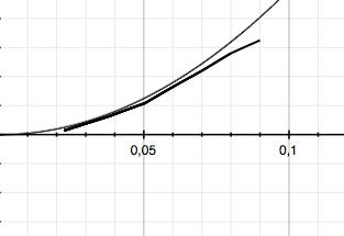
The idea behind this method is to approximate a curve by using short lines.

This is done by calculating the slope on a given point and drawing a short line with the same slope. At the end of this line, you calculate the slope again and draw another line. As you can see, the accuracy depends on the length of the lines.

Did you wonder what deltaT is used for?

The numerical algorithms you use have a step size, which is important for the accuracy of such algorithms; bigger step sizes cause lower accuracy but faster execution speed and vice versa.

deltaT is the step size for your algorithms. You initialized it with a value of 0.1, meaning that you calculated the position of the mass for every 0.1 second. In the case of the Euler method, this means that the lines have a length of 0.1 units on the x-Axis.

Before you start coding, you need to have a look again at the formula:

This second order differential equation can be replaced with two differential equations of first order.

can be written as and this as

You get this by using the difference quotient:

And you also get those:

With these equations, you can directly implement the Euler method.

Add the following code right behind solveExact:

func solveEuler(amplitude: Double, phase: Double, kSpring: Double, mass: Double, t: Double) {
  //1
  var x = amplitude * sin(phase)
  let omega = sqrt(kSpring / mass)
  var i = 0.0
  //2
  var v = amplitude * omega * cos(phase);
  var vold = v
  var xoldEuler = x
    
  while i < 100 {
    //3
    v -= omega * omega  * x * t
    //4
    x += vold * t
    xoldEuler = x
        
    vold = v
    i+=t
    }
}

What does this do?

1. Sets the current position and omega.
2. Calculates thee current speed.
3. Makes calculating the new velocity the first order of business inside the while loop.
4. The new position calculates at the end based on the velocity, and at the end, i is incremented by the step size t.

Now test this method by adding the following to the bottom of your playground:

osci.solveUsingSolver(solveEuler)

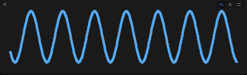
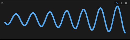
Then add a value history to the line xoldEuler = x. Take a look at the history, and you'll see that this method also draws a sine curve with a rising amplitude. The Euler method is not exact, and in this instance the big step size of 0.1 is contributing to the inaccuracy.

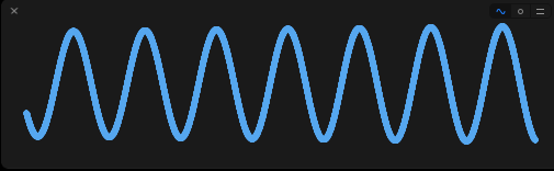
Here is another image, but this shows how it looks with a step size of 0.01, which leads to a much better solution. So, when you think about the Euler method, remember that it's most useful for small step sizes, but it also has the easiest implementation.

Velocity Verlet

The last method is called Velocity Verlet. It works off the same idea as Euler but calculates the new position a slightly different way.

Euler calculates the new position, while ignoring the actual acceleration, with the formula .

Velocity Verlet takes acceleration into account − this brings better results for the same step size.

Add the following code right after solveEuler:

func solveVerlet(amplitude: Double, phase: Double, kSpring: Double, mass: Double, t: Double) {
  //1
  var x = amplitude * sin(phase)
  var xoldVerlet = x
  let omega = sqrt(kSpring / mass)
    
  var v = amplitude * omega * cos(phase)
  var vold = v
  var i = 0.0
    
  while i < 100 {
    //2
    x = xoldVerlet + v * t + 0.5 * omega * omega * t * t
    v -= omega * omega * x * t
    xoldVerlet = x
    i+=t
  }
}

What's going on here?

1. Everything until the loop is the same as before.
2. Calculates the new position and velocity and increments i.

Again, test the function by adding this line to the end of your playground:

osci.solveUsingSolver(solveVerlet)

And also add a value history to the line xoldVerlet = x