Beginning Machine Learning with Keras & Core ML
In this Keras machine learning tutorial, you’ll learn how to train a convolutional neural network model, convert it to Core ML, and integrate it into an iOS app. By Audrey Tam.
Define Model Architecture

Model architecture is a form of alchemy, like secret family recipes for the perfect barbecue sauce or garam masala. You might start with a general-purpose architecture, then tweak it to exploit symmetries in your input data, or to produce a model with specific characteristics.
Here are models from two researchers: Sri Raghu Malireddi and François Chollet, the author of Keras. Chollet’s is general-purpose, and Malireddi’s is designed to produce a small model, suitable for mobile apps.
Enter the code below, and run it to see the model summaries.
Malireddi’s Architecture
model_m = Sequential()
model_m.add(Conv2D(32, (5, 5), input_shape=input_shape, activation='relu'))
model_m.add(MaxPooling2D(pool_size=(2, 2)))
model_m.add(Dropout(0.5))
model_m.add(Conv2D(64, (3, 3), activation='relu'))
model_m.add(MaxPooling2D(pool_size=(2, 2)))
model_m.add(Dropout(0.2))
model_m.add(Conv2D(128, (1, 1), activation='relu'))
model_m.add(MaxPooling2D(pool_size=(2, 2)))
model_m.add(Dropout(0.2))
model_m.add(Flatten())
model_m.add(Dense(128, activation='relu'))
model_m.add(Dense(num_classes, activation='softmax'))
# Inspect model's layers, output shapes, number of trainable parameters
print(model_m.summary())
Chollet’s Architecture
model_c = Sequential()
model_c.add(Conv2D(32, (3, 3), input_shape=input_shape, activation='relu'))
# Note: hwchong, elitedatascience use 32 for second Conv2D
model_c.add(Conv2D(64, (3, 3), activation='relu'))
model_c.add(MaxPooling2D(pool_size=(2, 2)))
model_c.add(Dropout(0.25))
model_c.add(Flatten())
model_c.add(Dense(128, activation='relu'))
model_c.add(Dropout(0.5))
model_c.add(Dense(num_classes, activation='softmax'))
# Inspect model's layers, output shapes, number of trainable parameters
print(model_c.summary())
Although Malireddi’s architecture has one more convolutional layer (Conv2D) than Chollet’s, it runs much faster, and the resulting model is much smaller.
Model Summaries
Take a quick look at the model summaries for these two models:
model_m:
Layer (type)                 Output Shape              Param #
=================================================================
conv2d_6 (Conv2D)            (None, 24, 24, 32)        832
_________________________________________________________________
max_pooling2d_5 (MaxPooling2 (None, 12, 12, 32)        0
_________________________________________________________________
dropout_6 (Dropout)          (None, 12, 12, 32)        0
_________________________________________________________________
conv2d_7 (Conv2D)            (None, 10, 10, 64)        18496
_________________________________________________________________
max_pooling2d_6 (MaxPooling2 (None, 5, 5, 64)          0
_________________________________________________________________
dropout_7 (Dropout)          (None, 5, 5, 64)          0
_________________________________________________________________
conv2d_8 (Conv2D)            (None, 5, 5, 128)         8320
_________________________________________________________________
max_pooling2d_7 (MaxPooling2 (None, 2, 2, 128)         0
_________________________________________________________________
dropout_8 (Dropout)          (None, 2, 2, 128)         0
_________________________________________________________________
flatten_3 (Flatten)          (None, 512)               0
_________________________________________________________________
dense_5 (Dense)              (None, 128)               65664
_________________________________________________________________
dense_6 (Dense)              (None, 10)                1290
=================================================================
Total params: 94,602
Trainable params: 94,602
Non-trainable params: 0
model_c:
Layer (type)                 Output Shape              Param #
=================================================================
conv2d_4 (Conv2D)            (None, 26, 26, 32)        320
_________________________________________________________________
conv2d_5 (Conv2D)            (None, 24, 24, 64)        18496
_________________________________________________________________
max_pooling2d_4 (MaxPooling2 (None, 12, 12, 64)        0
_________________________________________________________________
dropout_4 (Dropout)          (None, 12, 12, 64)        0
_________________________________________________________________
flatten_2 (Flatten)          (None, 9216)              0
_________________________________________________________________
dense_3 (Dense)              (None, 128)               1179776
_________________________________________________________________
dropout_5 (Dropout)          (None, 128)               0
_________________________________________________________________
dense_4 (Dense)              (None, 10)                1290
=================================================================
Total params: 1,199,882
Trainable params: 1,199,882
Non-trainable params: 0
The bottom line Total params is the main reason for the size difference: Chollet’s 1,199,882 is 12.5 times more than Malireddi’s 94,602. And that’s just about exactly the difference in model size: 4.8MB vs 380KB.
Malireddi’s model has three Conv2D layers, each followed by a MaxPooling2D layer, which halves the layer’s width and height. This makes the number of parameters for the first dense layer much smaller than Chollet’s, and explains why Malireddi’s model is much smaller and trains much faster. The implementation of convolutional layers is highly optimized, so the additional convolutional layer improves the accuracy without adding much to training time. But the smaller dense layer runs much faster than Chollet’s.
I’ll tell you about layers, output shape and parameter numbers in the Explanations section, while you wait for the next step to finish running.
Train the Model
Define Callbacks List
callbacks is an optional argument for the fit function, so define callbacks_list first.
Enter the code below, and run it.
callbacks_list = [
    keras.callbacks.ModelCheckpoint(
        filepath='best_model.{epoch:02d}-{val_loss:.2f}.h5',
        monitor='val_loss', save_best_only=True),
    keras.callbacks.EarlyStopping(monitor='acc', patience=1)
]
An epoch is a complete pass through all the mini-batches in the dataset.
The ModelCheckpoint callback monitors the validation loss value, saving the model with the lowest-so-far value in a file with the epoch number and the validation loss in the filename.
The EarlyStopping callback monitors training accuracy: if it fails to improve for two consecutive epochs, training stops early. In my experiments, this never happened: if acc went down in one epoch, it always recovered in the next.
Compile & Fit Model
Unless you have access to a GPU, I recommend you use Malireddi’s model_m for this step, as it runs much faster than Chollet’s model_c: on my MacBook Pro, 76-106s/epoch vs. 246-309s/epoch, or about 15 minutes vs. 45 minutes.
docker run command. Paste the URL or token into the browser or login page, navigate to the notebook, and click the Not Trusted button. Select this cell, then select Cell\Run All Above from the menu.
Enter the code below, and run it. This will take quite a while, so read the Explanations section while you wait. But check Finder after a couple of minutes, to make sure the notebook is saving .h5 files.
model_m.compile(loss='categorical_crossentropy',
                optimizer='adam', metrics=['accuracy'])

# Hyper-parameters
batch_size = 200
epochs = 10

# Enable validation to use ModelCheckpoint and EarlyStopping callbacks.
model_m.fit(
    x_train, y_train, batch_size=batch_size, epochs=epochs,
    callbacks=callbacks_list, validation_data=(x_val, y_val), verbose=1)
Convolutional Neural Network: Explanations
You can use just about any ML approach to create an MNIST classifier, but this tutorial uses a convolutional neural network (CNN), because that’s a key strength of TensorFlow and Keras.
Convolutional neural networks assume inputs are images, and arrange neurons in three dimensions: width, height, depth. A CNN consists of convolutional layers, each detecting higher-level features of the training images: the first layer might train filters to detect short lines or arcs at various angles; the second layer trains filters to detect significant combinations of these lines; the final layer’s filters build on the previous layers to classify the image.

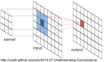
Each convolutional layer passes a small square kernel of weights — 1×1, 3×3 or 5×5 — over the input, computing the weighted sum of the input units under the kernel. This is the convolution process.
Each neuron is connected to only 1, 9, or 25 neurons in the previous layer, so there’s a danger of co-adapting — depending too much on a few inputs — and this can lead to overfitting. So CNNs include pooling and dropout layers to counteract co-adapting and overfitting. I explain these, below.
Sample Model
Here’s Malireddi’s model again:
model_m = Sequential()
model_m.add(Conv2D(32, (5, 5), input_shape=input_shape, activation='relu'))
model_m.add(MaxPooling2D(pool_size=(2, 2)))
model_m.add(Dropout(0.5))
model_m.add(Conv2D(64, (3, 3), activation='relu'))
model_m.add(MaxPooling2D(pool_size=(2, 2)))
model_m.add(Dropout(0.2))
model_m.add(Conv2D(128, (1, 1), activation='relu'))
model_m.add(MaxPooling2D(pool_size=(2, 2)))
model_m.add(Dropout(0.2))
model_m.add(Flatten())
model_m.add(Dense(128, activation='relu'))
model_m.add(Dense(num_classes, activation='softmax'))
Let’s work our way through this code.