Numerical Algorithms using Playgrounds

Taking Bisection to Playgrounds

At this point, you’re going to take the theory and put it into practice by creating your own bisection algorithm. Create a new playground and add the following function to it.

func bisection(x: Double) -> Double {
//1
    var lower = 1.0
    //2
    var upper = x
    //3
    var m = (lower + upper) / 2
    var epsilon = 1e-10
    //4
    while (fabs(m * m - x) > epsilon) {
    //5
        m = (lower + upper) / 2
        if m * m > x {
            upper = m
        } else {
            lower = m
        }
    }
    
    return m
}

What does each section do?

1. Sets the lower bound to 1
2. Sets the upper bound to x
3. Finds the middle and defines the desired accuracy
4. Checks if the operation has reached the desired accuracy
5. If not, this block finds the middle of the new interval and checks which interval to use next

To test this function, add this line to your playground.

let bis = bisection(2.5)

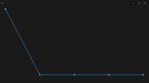
As you can see on the right of the line m = (lower + upper) / 2, this code executes 35 times, meaning this method takes 35 steps to find the result.

Now you’re going to take advantage of one of the loveable features of playgrounds — the ability to view the history of a value.

Since the bisection algorithm successively calculates more accurate approximations of the actual solution, you can use the value history graph to see how this numerical algorithm converges on the correct solution.

Press option+cmd+enter to open the assistant editor, and then click on the rounded button on the right side of the line m = (lower + upper) / 2 to add a value history to the assistant editor.

Here you can see the method jumping around the correct value.

Ancient Math Still Works

The next algorithm you’ll learn dates back to antiquity. It originated in Babylonia, as far back as 1750 B.C, but was described in Heron of Alexandria’s book Metrica around the year 100. And this is how it came to be known as Heron’s method. You can learn more about Heron’s method over here.

This method works by using the function , where a is the number for which you want to calculate the square root. If you can find this curve’s zero point — the value of x where the function equals zero — then you have found the square root of a.

To do this, you start with an arbitrary starting value of x, calculate the tangent line at this value, and then find the tangent line’s zero point. Then you repeat this using that zero point as the next starting value, and keep repeating until you reach the desired accuracy.

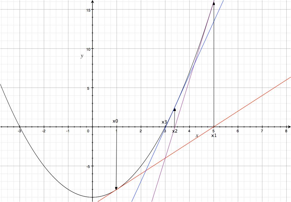
Since every tangent moves closer to true zero, the process converges on the true answer. The next graphic illustrates this process by solving with a=9, using a starting value of 1.

The starting point at x0=1 generates the red tangent line, producing the next point x1 that generates the purple line, producing the x2 that generates the blue line, finally leading to the answer.

Ancient Math, Meet Playgrounds

You have something that the Babylonians did not: playgrounds. Check out what happens when you add the following function to your playground:

func heron(x: Double) -> Double {
  //1
  var xOld = 0.0
  var xNew = (x + 1.0) / 2.0
  var epsilon = 1e-10
	
  //2
  while (fabs(xNew - xOld) > epsilon) {
    //3
    xOld = xNew
    xNew = (xOld + x / xOld) / 2
  }
   
  return xNew
}

What’s happening here?

• A good starting point for this method is found the way xNew is initialized.
• epsilon is the desired accuracy.
• In this case, you calculate the square root up to the 10th decimal place.

1. Creates variables to store the current result. xOld is the last calculated value andxNew the actual value.
2. While checks if the desired accuracy is reached.
3. If not, xNew becomes the new xOld, and then the next iteration starts.

Check your code by adding the line:

let her = heron(2.5)

Heron method requires only five iterations to find the result.

Click on the rounded button on the right side of the line xNew = (xOld + x / xOld) / 2 to add a value history to the assistant editor, and you’ll see that the first iteration found a good approximation.

Meet Harmonic Oscillators

In this section, you’ll learn how to use numerical integration algorithms in order to model a simple harmonic oscillator, a basic dynamical system.

The system can describe many phenomena, from the swinging of a pendulum to the vibrations of a weight on a spring, to name a couple. Specifically, it can be used to describe scenarios that involve a certain offset or displacement that changes over time.

You’ll use the playground’s value history feature to model how this offset value changes over time, but won’t use it to show how your numerical approximation takes you successively closer to the perfect solution.

For this example, you’ll work with a mass attached to a spring. To make things easier, you’ll ignore damping and gravity, so the only force acting on the mass is the spring force that tries to pull the mass back to an offset position of zero.

With this assumption, you only need to work with two physical laws.

• Newton’s Second Law: , which describes how the force on the mass changes its acceleration.
• Hook’s Law:, which describes how the spring applies a force on the mass proportional to its displacement, where k is the spring constant and x is the displacement.

Harmonic Oscillator Formula

Since the spring is the only source of force on the mass, you combine these equations and write the following:

You can write this as:

is also known as , which is the square of the resonance frequency.

The formula for the exact solution is as follows:

A is the amplitude, and in this case it means the displacement, , is known as phase difference. Both are constant values that can be found using initial values.

If you say at the time t=0 you have and you find the amplitude and phase difference as:

Let’s look at an example. We have a mass of 2kg attached to a spring with a spring constant k=196N/m. At the time t=0 the spring has a displacement of 0.1m. To calculate and we have to calculate .

and