Swift Algorithm Club: Strassen’s Algorithm
In this tutorial, you’ll learn how to implement Strassen’s Matrix Multiplication in Swift. This was the first matrix multiplication algorithm to beat the naive O(n³) implementation, and is a fantastic example of the Divide and Conquer coding paradigm — a favorite topic in coding interviews. By Richard Ash.
The Swift Algorithm Club, also known as SAC, is a community-driven open-source project that contributes to building popular algorithms and data structures in Swift.
Every month, the SAC team will feature a data structure or algorithm from the club in a tutorial on this site. If you want to learn more about algorithms and data structures, follow along with us!
This tutorial assumes you have read the following tutorials (or have equivalent knowledge):
Getting Started
In this tutorial, you’ll learn how to implement Strassen’s Matrix Multiplication. It was developed by Volker Strassen, a German mathematician, in 1969 and was the first to beat the naive O(n³) implementation. In addition, Strassen’s algorithm is a fantastic example of the Divide and Conquer coding paradigm — a favorite topic in coding interviews.
Specifically, you will:
- Learn the applications of matrix multiplication and how it works.
- Implement a naive implementation.
- Implement Strassen’s algorithm and learn how it differs from the naive approach.
But, first, a little theory!
Understanding Matrix Multiplication
Matrix multiplication is an operation that combines two matrices together. It is incredibly useful, having applications across physics, engineering and mathematics! Some real-world examples include:
1. Google’s PageRank algorithm
2. Graph computations
3. Physical simulations
How Does It Work?
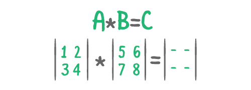
To see how matrix multiplication works, consider the following example:

To start, you’re multiplying two 2×2 matrices A and B.
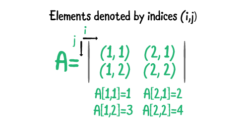
Each element of matrix A is denoted by a combination of the indices (i, j). Both i and j start from 1 at the top-left corner of the matrix and increase by one until the final row and column. You denote the element at row i and column j by writing A[i, j]. Because matrix A has two rows and two columns, there are four index combinations:
1. A[1, 1] is equal to the element at the first row (i = 1) and the first column (j = 1).
2. A[2, 1] is the element at the second row (i = 2) and the first column (j = 1).
3. A[1, 2] is the element at the first row (i = 1) and the second column (j = 2).
4. A[2, 2] is the element at the second row (i = 2) and the second column (j = 2).
Challenge
Write out each combination of indices i and j for matrix B. Include the element at each combination.
[spoiler title=”Solution”]
B[1, 1] = 5
B[1, 2] = 6
B[2, 1] = 7
B[2, 2] = 8
[/spoiler]
The result of multiplying A and B is a new matrix: C. C’s elements are determined by taking the dot product of A’s i row with the B’s j column.
You’ll examine this operation in detail by filling in the four elements of C:
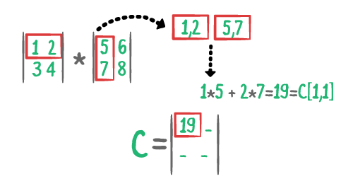
1. [i=1, j=1]: The element at [1, 1] is the dot product of A’s first row and B’s first column. Because A’s first row is [1, 2] and B’s first column is [5, 7], you multiply 1 by 5 and 2 by 7. You then add the results together to get 19.
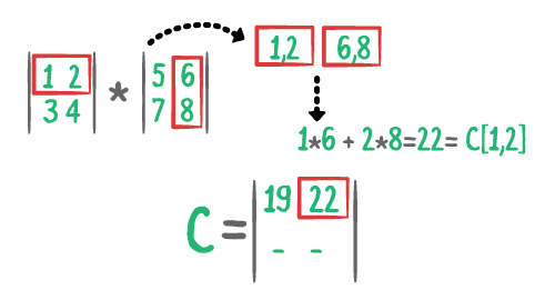
2. [i=1, j=2]: Because i=1 and j=2, this component will represent the upper-right element in your new matrix, C. A’s first row is [1, 2] and B’s second column is [6, 8]. You multiply 1 by 6 and 2 by 8. You then add the results together to get 22.
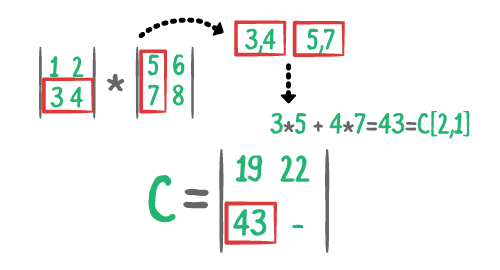
3. [i=2, j=1]: A’s second row is [3, 4] and B’s first column is [5, 7]. Multiply 3 by 5 and 4 by 7; add those results together to get 43.
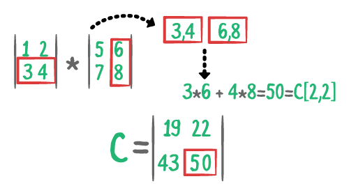
4. [i=2, j=2]: A’s second row is [3, 4] and B’s second column is [6, 8]. By multiplying 3 by 6 and 4 by 8, then adding those results together, you get 50.
Phew, good job! That was a lot of work.
Multiplying Matrices Correctly
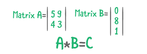
For a matrix multiplication to be valid, the first matrix needs to have the same number of columns as the second matrix has number of rows. In math terminology, if matrix A’s dimensions are m × n, then matrix B’s dimensions need to be n × p. The result matrix C must be m × p. Look at an example in which this is not the case:
You can use the same method as above:
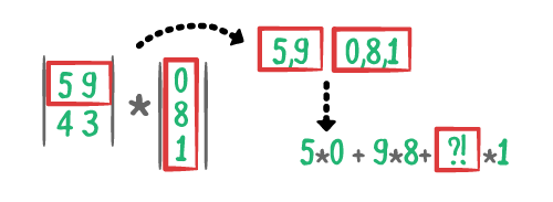
1. [i=1, j=1]: A’s first row is [5, 9] and B’s first column is [0, 8, 1]. Multiply 5 by 0 and 9 by 8 and …?!?! There’s no third number from A’s first row to multiply by! You can check the result on WolfphramAlpha. This error is called incompatible dimensions. A’s first row and B’s first column are different lengths; you cannot take their dot product and therefore can’t complete the matrix multiplication.
Now for practice — try this next one on your own! :]
Challenge
Multiply the following matrices:
Matrix A:
1 8
9 0
21 -2

Matrix B:
5 2
2 4
[spoiler title=”Solution”]
[i=1, j=1]:
A's first row = [1, 8]
B's first column = [5, 2]
[1, 8] dot [5, 2] = [1*5 + 8*2] = [21] = C[1, 1]
[i=1, j=2]:
A's first row = [1, 8]
B's second column = [2, 4]
[1, 8] dot [2, 4] = [1*2 + 8*4] = [34] = C[1, 2]
[i=2, j=1]:
A's second row = [9, 0]
B's first column = [5, 2]
[9, 0] dot [5, 2] = [9*5 + 0*2] = [45] = C[2, 1]
[i=2, j=2]:
A's second row = [9, 0]
B's second column = [2, 4]
[9, 0] dot [2, 4] = [9*2 + 0*4] = [18] = C[2, 2]
[i=3, j=1]:
A's third row = [21 -2]
B's first column = [5, 2]
[21, -2] dot [5, 2] = [21*5 + -2*2] = [101] = C[3,1]
[i=3, j=2]:
A's third row = [21, -2]
B's second column = [2, 4]
[21, -2] dot [2, 4] = [21*2 + -2*4] = [34] = C[3, 2]
Matrix C:
21 34
45 18
101 34
[/spoiler]
Aren’t you tired of doing matrix multiplication by hand? Let’s now look at how you can write this up in code!