Machine Learning: End-to-end Classification

In machine learning, classification is the task of predicting the class of an object out of a finite number of classes, given some input labeled dataset. For example, you might have a list of 10,000 emails and the need to determine whether or not they’re spam. You would train a classifier on this input data and it would be able to predict if a new email is spam or not. Another classic example is a classifier that can predict what object is depicted in an image from a list of known classes such as house, car, cat and so on.

In this tutorial, you’ll learn how to:

• Preprocess and prepare data to feed into a machine learning classification algorithm.
• Evaluate your classifier against the most commonly used classification metrics.
• Optimize the parameters of a machine learning classifier.

Getting Started

Downloaded the materials for this tutorial using the Download Materials button at the top or bottom of this page. Copy the two ipynb files to your Jupyter Notebooks folder. Then, open Starter.ipynb with Jupyter.

From the top menu of Jupyter, select Kernel, and then Restart & Run All:

Select Restart and Run All Cells if prompted to “Restart kernel and re-run the whole notebook”.

The bottom cell contains code to download a dataset called credit. This dataset contains 400 rows wherein each row contains some credit-related information about a person as well as some personal details such as age and student status. You can see the first 5 rows in the notebook.

Your goal in this project is to use this dataset to create a classifier to predict whether or not a user is creditworthy, using as little personal information as possible. You define a creditworthy person as someone who has a credit score (rating) of over 600.

Preprocessing and Selecting Features

The first step to any machine learning project is cleaning or transforming the data into a format that can be used by machine learning algorithms. In most cases, you’ll need numerical data without any missing values or outliers that might make it much harder to train a model.

In the case of the credit dataset, the values are already very cleaned up, but you still need to transform the data into numerical values.

Encoding Labels

One of the simplest forms of preprocessing steps is called label encoding. It allows you to convert non numeric values to numeric values. You’ll use it to convert the Student, Married, and Gender columns.

Add the following code to a new cell just below, “Your code goes below here”:

# 1
credit_ = credit.copy()

# 2
credit_["Student"] = credit["Student"].map(lambda student: 1 if student == "Yes" else 0)

credit_["Married"] = credit["Married"].map(lambda married: 1 if married == "Yes" else 0)

# 3
credit_["Female"] = credit["Gender"].map(lambda gender: 1 if gender == "Female" else 0)
credit_.drop("Gender", axis=1, inplace=True)

# 4
credit_.head()

Here’s what’s happening in the code above:

1. You make a copy of the credit dataset to be able to cleanly transform the dataset. credit_ will hold the ready-to-use data after processing is complete.
2. For Student and Married, you label encode Yes to 1 and No to 0.
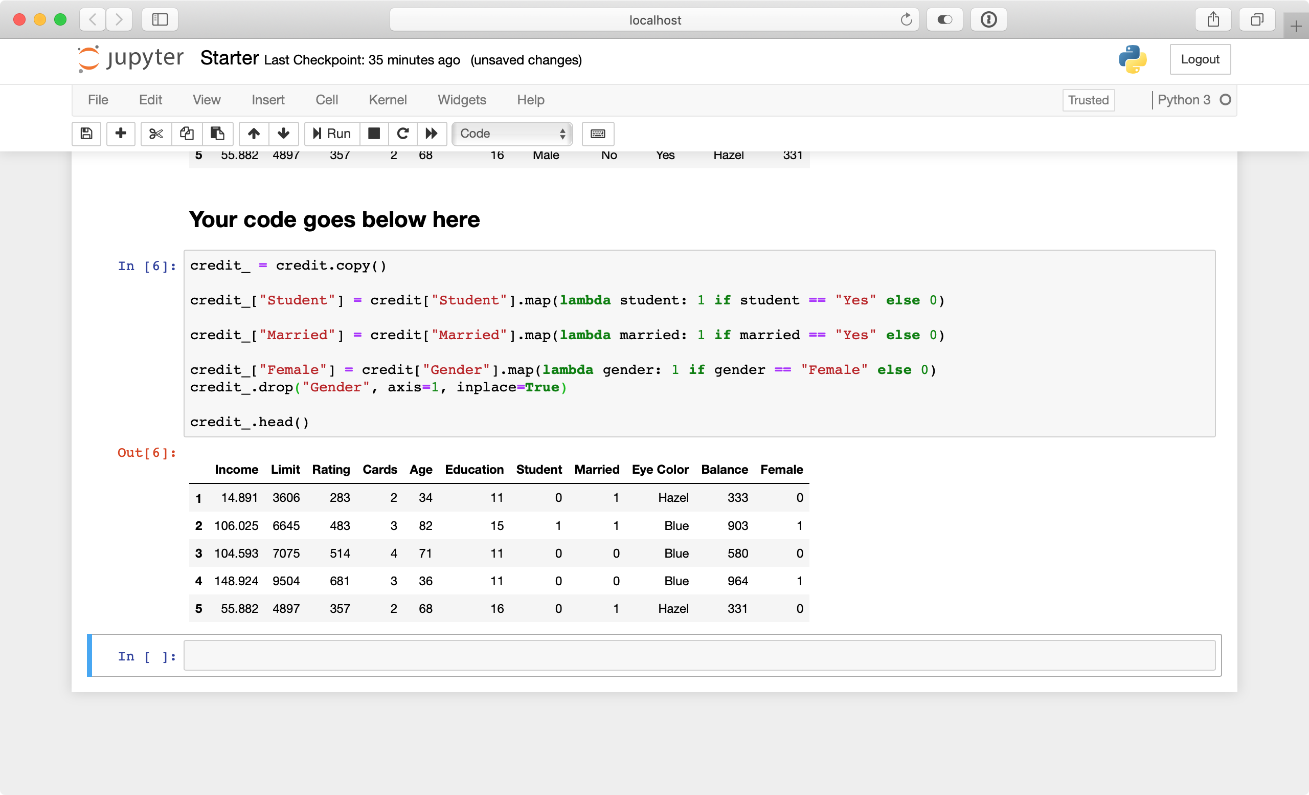
3. Here, you also do the same for the Gender field, while renaming the column to Female. You also drop the Gender column afterwards.
4. At the end of the cell, you display the top rows from the data to verify your processing steps were successful.

Press Control+Enter to run your code. It should look similar to the following:

So far so good! You might be thinking about doing the same to the Eye Color column. This column holds three values: Green, Blue and Hazel. You could replace these values with 0, 1, and 2, respectively.

Most machine learning algorithms will misinterpret this information though. An algorithm like logistic regression would learn that Eye Color with value 2, will have a stronger effect than 1. A much better approach is using one-hot encoding.

One-Hot Encoding

When using one-hot encoding, also called Dummy Variables, you create as many columns as there are distinct values. Each column then becomes 0 or 1, depending on if the original value for that row was equal to the new column or not. For example, if the row’s value is Blue, then in the one-hot encoded data, the Blue column would be 1, then both the Green, and Hazel columns would be 0.

To better visualize this, create a new cell by choosing Insert ▸ Insert Cell Below from the top menu and add the following code to the new cell:

pd.get_dummies(credit_["Eye Color"])

get_dummies will create dummy variables from the values observed in Eye Color. Run the cell to check it out:

Because the first entry in your dataset had hazel eyes, the first result here contains a 1 in Hazel and 0 for Blue and Green. The remaining 399 entries work the same way!

Go to Edit ▸ Delete Cells to delete the last cell. Next, add the following lines just before credit_.head() in the latest cell:

eye_color = pd.get_dummies(credit["Eye Color"], drop_first=True)
credit_ = pd.concat([credit_.drop("Eye Color", axis=1), eye_color], axis=1)

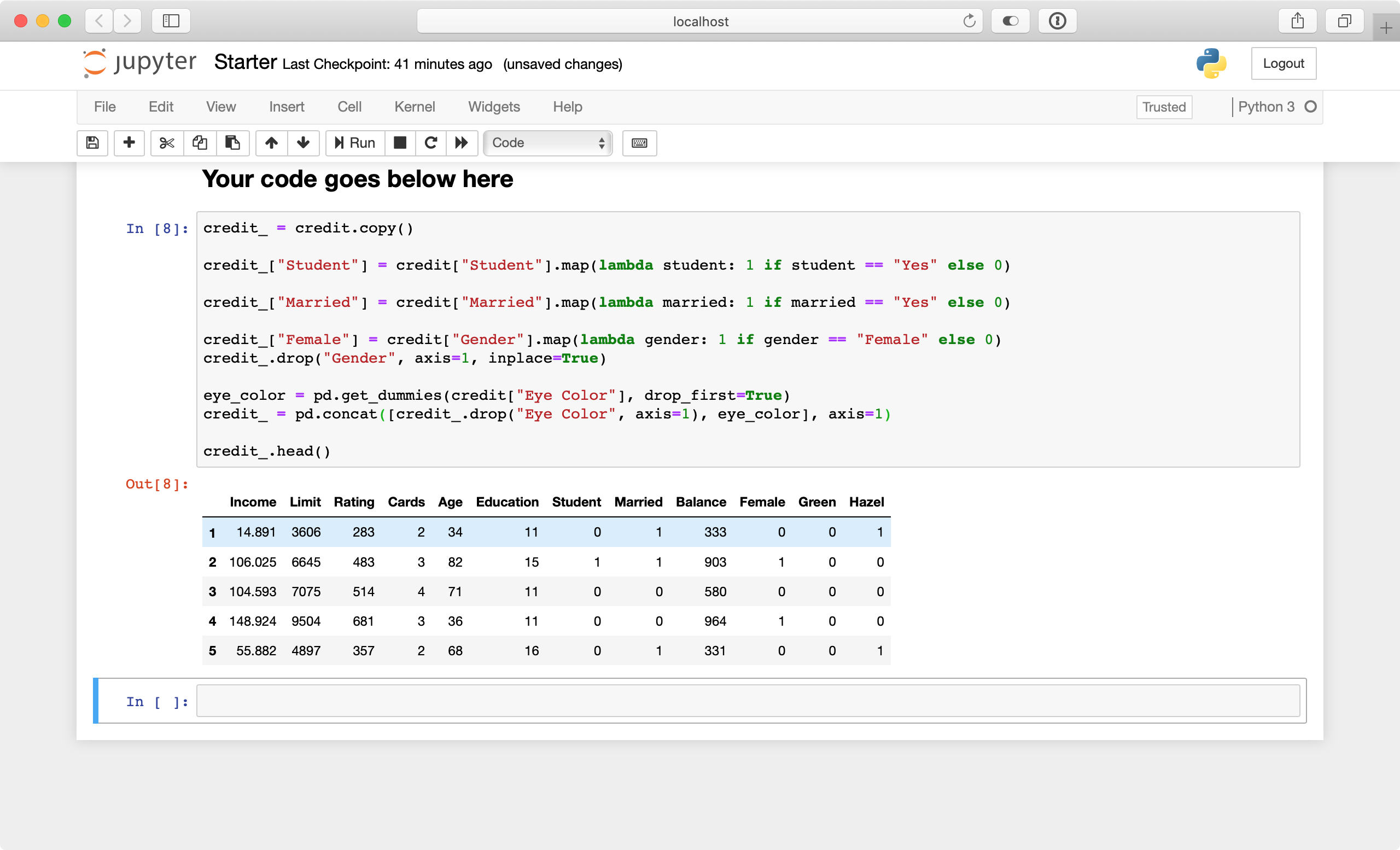
In the first line, you create the dummy columns for Eye Color while using drop_first=True to discard the first dummy column. You do this to save space because the last value can be inferred from the other two.

Then, you use concat to concatenate the dummy columns to the data frame at the end. Run the cell again and look at the results!

Target Label

For the last step of preprocessing, you’re going to create a target label. This will be the column your classifier will predict — in this case, whether or not the person is creditworthy.

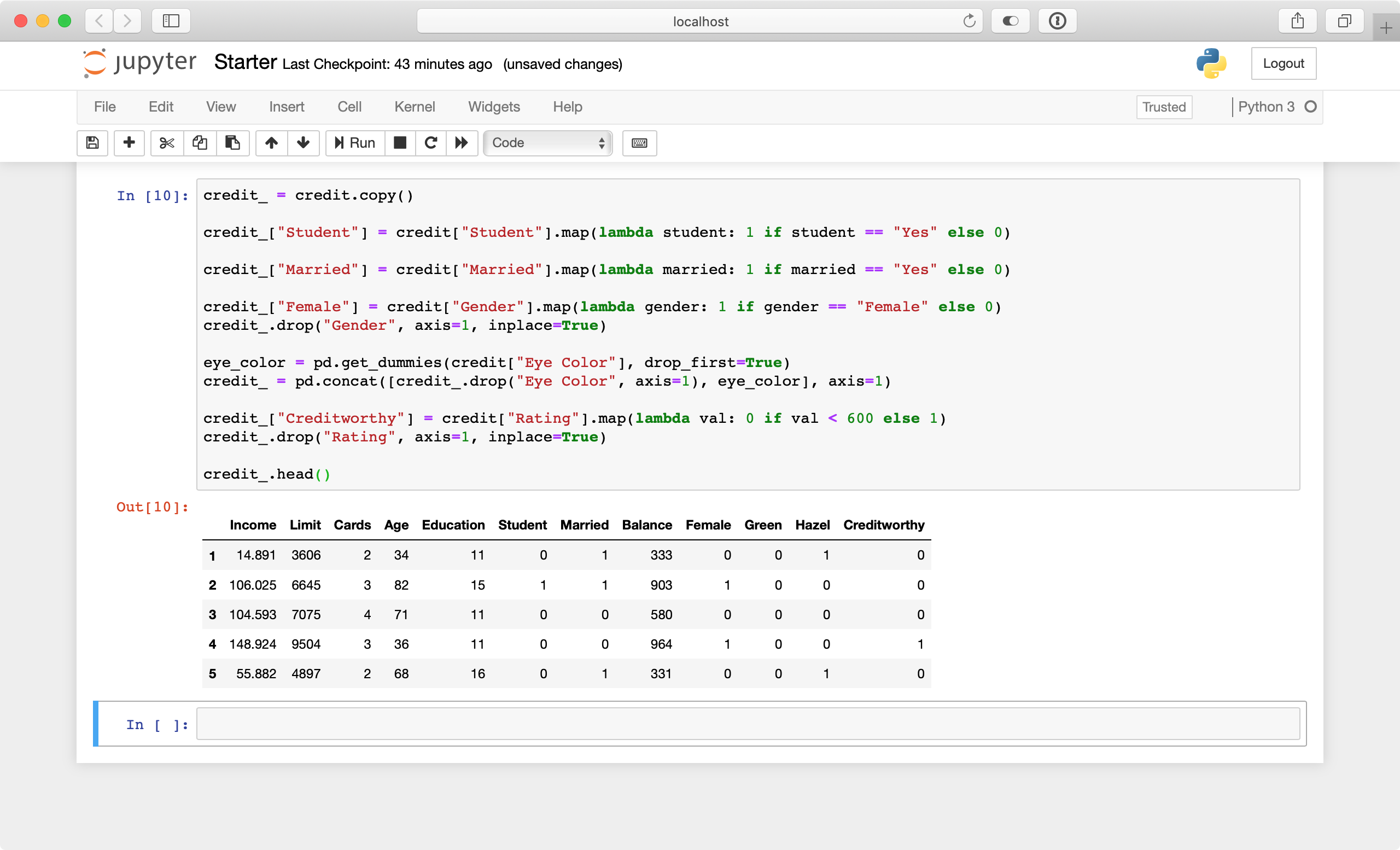
For a Rating greater than 600, the label will be 1 (creditworthy). Otherwise, you set it to 0. Add the following code to the current cell before credit_.head() again:

credit_["Creditworthy"] = credit["Rating"].map(lambda val: 0 if val < 600 else 1)
credit_.drop("Rating", axis=1, inplace=True)

This last column will be the column your classifier will predict, using a combination of the other columns.

Run this cell one last time. The preprocessing is now complete and your data frame is ready for training!